Welcome to Linear Models

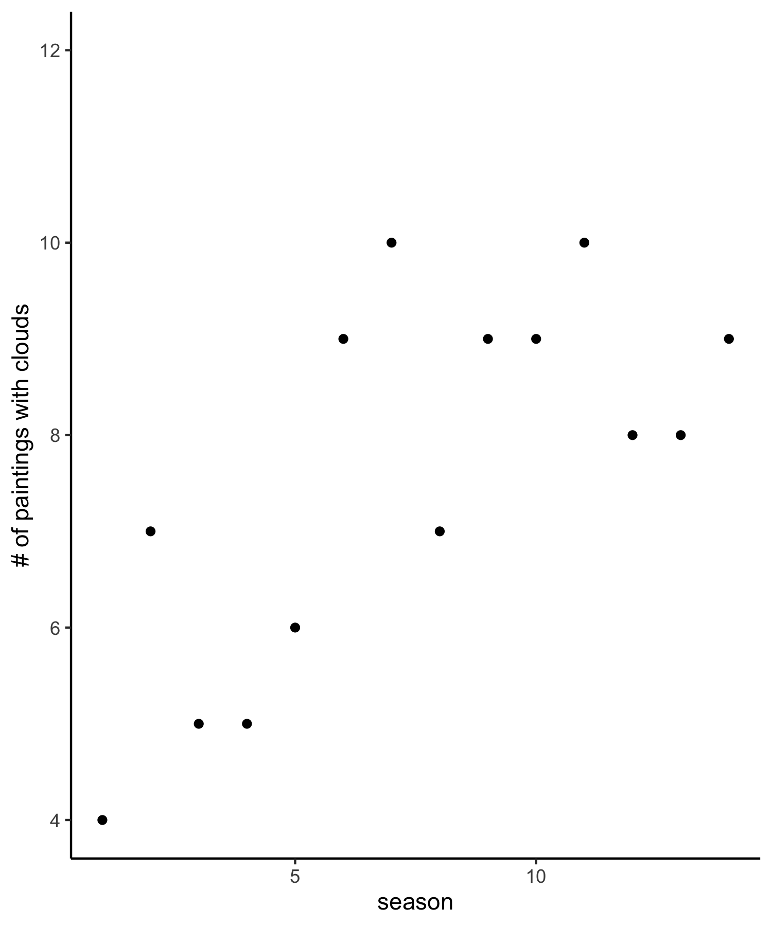
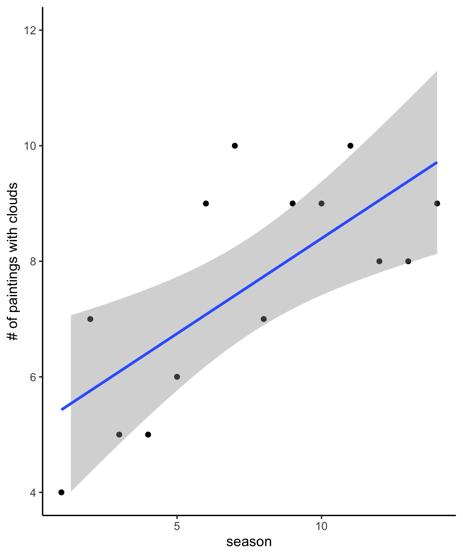
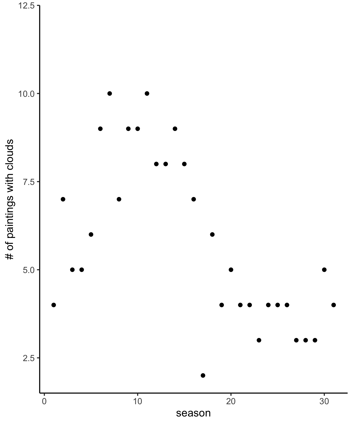
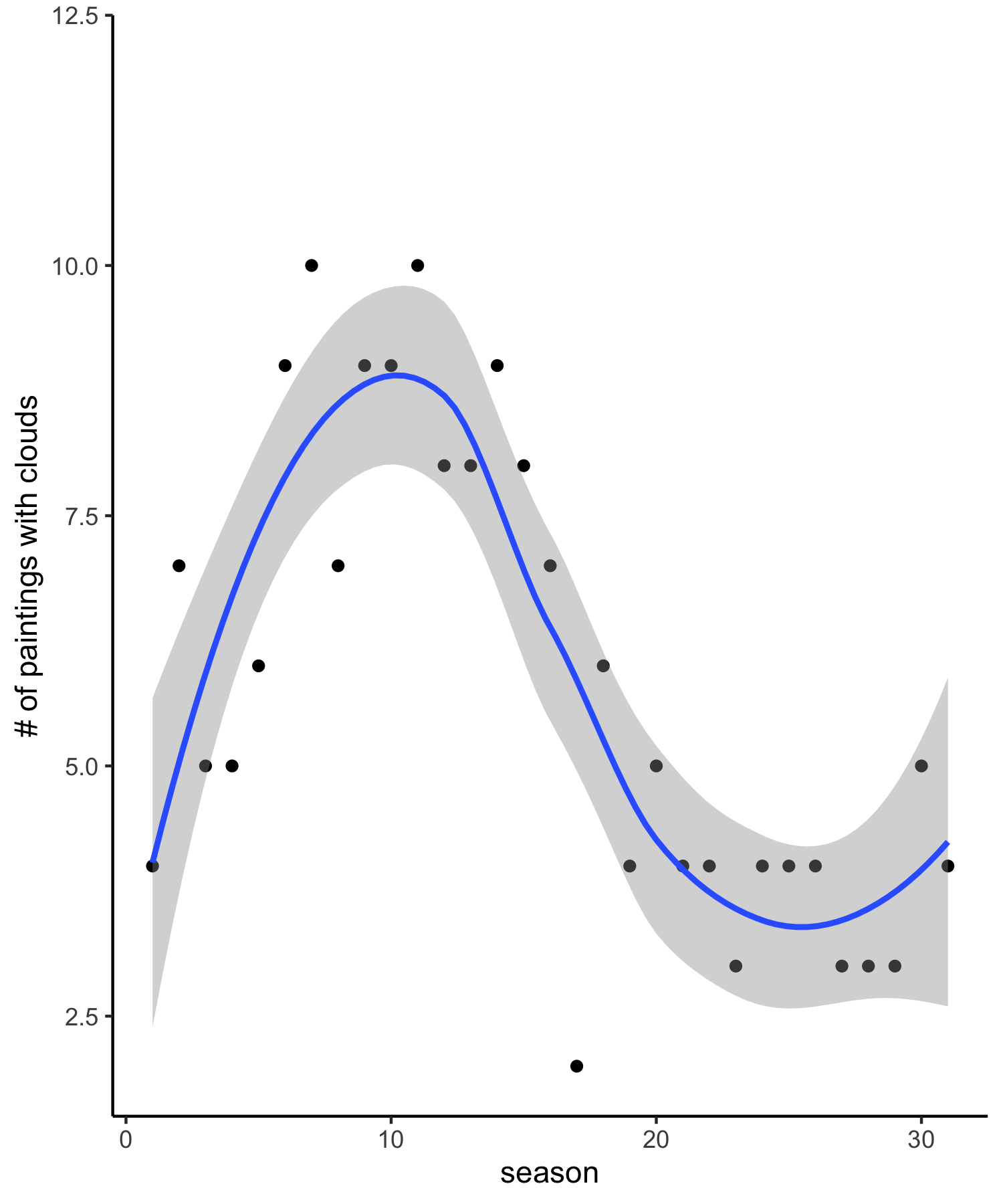
# Welcome to Linear Models
### Dr. D’Agostino McGowan

---

<div class="my-footer">
 
 Dr. Lucy D'Agostino McGowan

</div>

---

## 👋

##  Lucy D'Agostino McGowan

&nbsp; [mcgowald@wfu.edu](mailto:mcgowald@wfu.edu) 
 &nbsp; Tues/Thurs 9:30a-10:45a, 12:30p-1:45p

---

Everything you will need will be posted at:

# [bit.ly/sta-312-f20](http://bit.ly/sta-312-f20)

---
class: center, middle

### "truth … is much too complicated to allow anything but approximations" - John von Neumann

<img src = "https://farkasdilemma.files.wordpress.com/2013/01/vonneumann.png" height = "350"> </img>

John von Neumann, wearer of funny hats via <a href = "https://farkasdilemma.wordpress.com/2013/01/04/john-von-neumannm-wearer-of-funny-hats/"> farkasdilemma.wordpress.com</a>

---

### "Statistics is using data and knowledge about randomness to condense, communicate, and contextualize information and provide insight into the setting from which the data came." - Jo Hardin

Jo Hardin <a href = "https://research.pomona.edu/johardin/files/2012/08/jo_headshot3-3.png"> https://research.pomona.edu/johardin/</a>

---
class: center, middle

### "All models are wrong, but some are useful" - George Box

<img height="400" alt="GeorgeEPBox" src="https://upload.wikimedia.org/wikipedia/commons/thumb/a/a2/GeorgeEPBox.jpg/256px-GeorgeEPBox.jpg"></img>

DavidMCEddy at en.wikipedia <a href = "https://creativecommons.org/licenses/by-sa/3.0"> CC BY-SA 3.0 </a>, via Wikimedia Commons

---

---

# 🗣 math speak

---

# model

---

# data (to build the model)

---

# data (outcome)

---

# Simple Linear Regression

---

![](https://upload.wikimedia.org/wikipedia/en/7/70/Bob_at_Easel.jpg)

Bob at Easel from <a href = "https://en.wikipedia.org/wiki/File:Bob_at_Easel.jpg">Wikipedia</a>
---

]
.pull-right[
![](01-welcome_files/figure-html/unnamed-chunk-2-1.png)
]

### Data: [FiveThirtyEight](https://fivethirtyeight.com/features/a-statistical-analysis-of-the-work-of-bob-ross/)

---

]
.pull-right[
![](01-welcome_files/figure-html/unnamed-chunk-3-1.png)
]
---

]
.pull-right[
![](01-welcome_files/figure-html/unnamed-chunk-4-1.png)
]

---

]
.pull-right[
![](01-welcome_files/figure-html/unnamed-chunk-5-1.png)
]

.question[
 $$ 
 \text{# of paintings with clouds} = \color{blue}{\beta_0 + \beta_1 season
 }+ \epsilon 
 $$
]
---

]
.pull-right[
![](01-welcome_files/figure-html/unnamed-chunk-6-1.png)
]

.question[
 $$ 
 \text{# of paintings with clouds} = \color{blue}{\beta_0 + \beta_1 season
 }+ \epsilon 
 $$
]
---

]
.pull-right[
![](01-welcome_files/figure-html/unnamed-chunk-7-1.png)
]

.question[
 $$ 
 \text{# of paintings with clouds} = \color{blue}{\beta_0 + \beta_1 f(season)
 }+ \epsilon 
 $$
]
---

# Multiple Linear Regression

---
class: center, middle

# Let's go!

---

## Log into RStudio Pro

- **Note:** if you are off campus, you will need to use a [VPN to connect](https://is.wfu.edu/services/vpn/)
- Go to [rstudio.hpc.ar53.wfu.edu:8787](rstudio.hpc.ar53.wfu.edu:8787)
- Your username is your WFU username (typically the first part of your email)
- The password is: **R2D2Star!**

---

## `Penguin fun!`

- Once you log on to RStudio Pro, find the project `01-welcome-penguins`, click it
- In the Files pane in the bottom right corner, spot the file called `welcome-penguins.Rmd`. Open it, and then click on the "Knit" button. 
- Go back to the file and change your name on top (in the `yaml` -- we'll talk about what this means later) and knit again.
- Then, scroll to the `plot` chunk, below **Palmer Penguins**. Instead of looking at the relationship between flipper length and bill length, plot the relationship between flipper length and bill **depth**. _Hint, look at the full dataset at the bottom of the document for variable names, update the captions to match your new plot_. Knit again & voila!

---