class: center, middle, inverse, title-slide # Checking Error Assumptions ### Dr. D’Agostino McGowan --- layout: true <div class="my-footer"> <span> Dr. Lucy D'Agostino McGowan </span> </div> --- ## What are the assumptions for linear regression with respect to `\(\epsilon\)`? -- * Constant Variance -- * Normality -- * Independence --- ## Checking Normality * Hypothesis tests and confidence intervals rely on the errors being normally distributed -- * We can check the distribution of the _residuals_ using a Q-Q plot and a histogram --- ## Q-Q plot * Plot the sorted residuals against `\(\Phi^{-1}\left(\frac{i}{n+1}\right)\)` for `\(i = 1, \dots, n\)` -- ```r e <- resid(lm(mpg ~ disp, data = mtcars)) # get the residuals e <- e[order(e)] # sort n <- nrow(mtcars) # calculate n q <- qnorm(1:n/(n + 1)) # calculate q ``` --- ## Q-Q plot * Plot the sorted residuals against `\(\Phi^{-1}\left(\frac{i}{n+1}\right)\)` for `\(i = 1, \dots, n\)` ```r *e <- resid(lm(mpg ~ disp, data = mtcars)) # get the residuals e <- e[order(e)] # sort n <- nrow(mtcars) # calculate n q <- qnorm(1:n/(n + 1)) # calculate q ``` --- ## Q-Q plot * Plot the sorted residuals against `\(\Phi^{-1}\left(\frac{i}{n+1}\right)\)` for `\(i = 1, \dots, n\)` ```r e <- resid(lm(mpg ~ disp, data = mtcars)) # get the residuals *e <- e[order(e)] # sort n <- nrow(mtcars) # calculate n q <- qnorm(1:n/(n + 1)) # calculate q ``` --- ## Q-Q plot * Plot the sorted residuals against `\(\Phi^{-1}\left(\frac{i}{n+1}\right)\)` for `\(i = 1, \dots, n\)` ```r e <- resid(lm(mpg ~ disp, data = mtcars)) # get the residuals e <- e[order(e)] # sort *n <- nrow(mtcars) # calculate n q <- qnorm(1:n/(n + 1)) # calculate q ``` --- ## Q-Q plot * Plot the sorted residuals against `\(\Phi^{-1}\left(\frac{i}{n+1}\right)\)` for `\(i = 1, \dots, n\)` ```r e <- resid(lm(mpg ~ disp, data = mtcars)) # get the residuals e <- e[order(e)] # sort n <- nrow(mtcars) # calculate n *q <- qnorm(1:n/(n + 1)) # calculate q d <- data.frame( e = e, q = q ) ``` --- ## Q-Q plot * "by hand" .small[ ```r library(ggplot2) ggplot(d, aes(x = q, y = e)) + geom_point() ``` <!-- --> ] --- ## Q-Q plot * Let ggplot do the heavy lifting .small[ ```r ggplot(d, aes(sample = e)) + geom_qq() + geom_qq_line() ``` <!-- --> ] --- ## Q-Q plot * Let ggplot do the heavy lifting .small[ ```r *ggplot(d, aes(sample = e)) + geom_qq() + geom_qq_line() ``` <!-- --> ] --- ## Q-Q plot * Let ggplot do the heavy lifting .small[ ```r ggplot(d, aes(sample = e)) + * geom_qq() + geom_qq_line() ``` <!-- --> ] --- ## Q-Q plot * Let ggplot do the heavy lifting .small[ ```r ggplot(d, aes(sample = e)) + geom_qq() + * geom_qq_line() ``` <!-- --> ] --- ## Histogram ```r ggplot(d, aes(x = e)) + geom_histogram(bins = 15) ``` <!-- --> --- ## Generate a normal one ```r set.seed(1) e <- rnorm(1000) # generate some normally distributed errors e <- e[order(e)] d <- data.frame(e) ``` --- ## Normal Q-Q plot ```r ggplot(d, aes(sample = e)) + geom_qq() + geom_qq_line() ``` <!-- --> --- ## Normal Histogram ```r ggplot(d, aes(e)) + geom_histogram(bins = 20) ``` <!-- --> --- ## Skewed Right .small[ ```r e_right <- c(e[e > 0] * 5, e) ## generate right skewed data d <- data.frame(e_right) ggplot(d, aes(x = e_right)) + geom_histogram(bins = 30) ``` <!-- --> ] --- ## Skewed Right .small[ ```r ggplot(d, aes(sample = e_right)) + geom_qq() + geom_qq_line() ``` <!-- --> ] --- ## Skewed Left .small[ ```r e_left <- c(e[e < 0] * 5, e) ## generate left skewed data d <- data.frame(e_left) ggplot(d, aes(x = e_left)) + geom_histogram(bins = 30) ``` <!-- --> ] --- ## Skewed Left .small[ ```r ggplot(d, aes(sample = e_left)) + geom_qq() + geom_qq_line() ``` 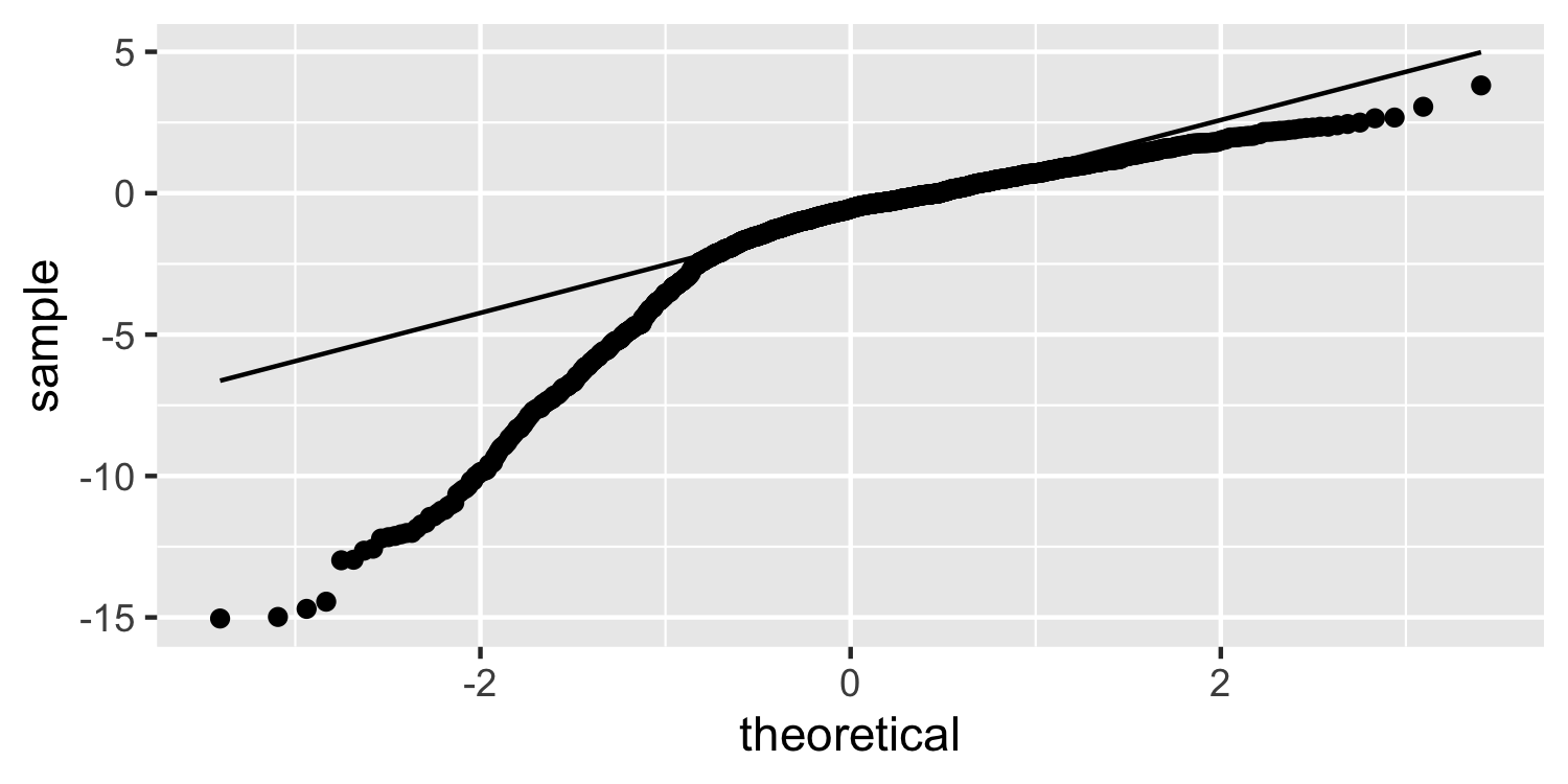<!-- --> ] --- class: inverse ## <svg style="height:0.8em;top:.04em;position:relative;" viewBox="0 0 640 512"><path d="M512 64v256H128V64h384m16-64H112C85.5 0 64 21.5 64 48v288c0 26.5 21.5 48 48 48h416c26.5 0 48-21.5 48-48V48c0-26.5-21.5-48-48-48zm100 416H389.5c-3 0-5.5 2.1-5.9 5.1C381.2 436.3 368 448 352 448h-64c-16 0-29.2-11.7-31.6-26.9-.5-2.9-3-5.1-5.9-5.1H12c-6.6 0-12 5.4-12 12v36c0 26.5 21.5 48 48 48h544c26.5 0 48-21.5 48-48v-36c0-6.6-5.4-12-12-12z"/></svg> `Application Exercise` Generate some "fake" residuals under the following scenarios and plot the Q-Q plot and histogram for each. Describe what you see. 1. Left-skewed data 2. Right-skewed data 3. Data generated under a lognormal distribution (use the `rlnorm()` function) 4. Data generated under a t-distribution with 2 degrees of freedom (use the `rt()` function) --- ## Correlated Errors * There is not a _single_ check for correlated errors since there so many different ways errors can be correlated -- * Examples: * Data collected over time * Spatial data * Data collected in blocks (for example eyes!) --- ## "Solving" these problems * **Constant Variance** -- * This can sometimes be resolved by fitting your model differently, perhaps incorporating _transformations_ (for example you could try to take the log of the outcome, y) -- * Another fix is **weighted least squares** --- ## "Solving" these problems * **Normality** -- * Appealing to the _central limit theorem_ if you have a large enough data set we don't have to worry as much about normality since our confidence intervals will be approximately correct -- * For skewed distributions, transformations can help -- * Check for constant variance (and linearity) first --- ## "Solving" these problems * **Correlated Errors** -- * You need to update the **structure** of the model * **generalized least squares**